Advanced concept maps#

Concept maps are not just simple tools. NASA for example used the IHMC concept mapping software (described in module 6) to model pages and pages of knowledge relating to the recent Mars Rovers exploration program. Other scientists use various forms of concept maps to help decode the human genome (DNA). In this module, I introduce you to some more advanced forms of concept maps, including:

• Systems concept maps. These model natural and man-made systems in which there is often no start or end point. They’re cyclical, and their real subject is feedback – the loops by which a system regulates itself. This is the lens of systems thinking and cybernetics.

• Decision Trees. These lay out a decision and its uncertain outcomes so you can weigh the options – including putting numbers on them where the payoffs and probabilities are known.

• Logic Trees. These use deductive and inductive reasoning to help you lay out and pressure-test an argument.

• Software-Based concept maps. The frontier of concept maps. See how concept maps are changing the way we interact with knowledge via computers.

• Other types of maps. Some examples of other types of specific concept maps.

Systems concept maps#

A systems concept map organizes information in a format that’s similar to a circular flowchart. It shows a cycle, or several cycles, in a system. The defining feature is that, unlike a flowchart, there’s often no start or end point – the arrows close back on themselves into a loop. That loop is the whole point, because it’s where feedback lives.

In the following basic example adapted from Peter Senge’s book The Fifth Discipline, the map shows how each element in the simple act of filling a bucket from a hose influences the others. Your perception of how full the bucket is sets the gap between where the water is and where you want it; that gap influences how far you open the faucet; the faucet sets the flow; the flow raises the level; and the new level changes your perception of the gap again. You keep going round this loop until the bucket is full.

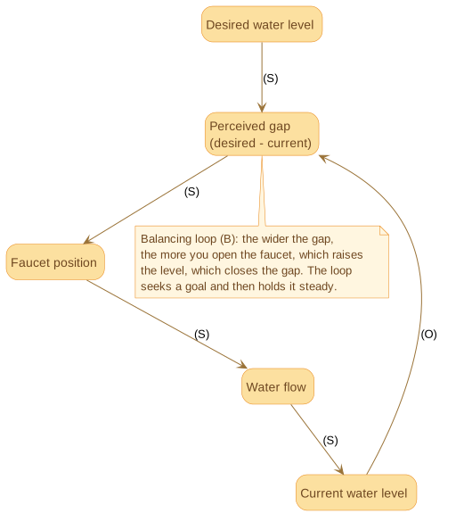
This is a balancing feedback loop – the most important idea in the whole module. The loop has a goal (the bucket full), and every time round it acts to close the gap between where things are and where you want them. When the gap is large you open the faucet wide; as the level approaches the goal you ease off; once it’s there, the loop holds it steady. Balancing loops are how systems regulate themselves, from a thermostat holding a room temperature to your body holding its blood sugar. Engineers call this negative feedback, and the broader study of such self-regulating, goal-seeking systems is cybernetics. You’re already doing it without thinking: filling a bucket is not a linear task but a control loop your brain evaluates several times a second.

The same lens explains why it’s so hard to get the shower temperature right. There’s a delay between turning the tap and feeling the result. With a delay in the loop, you can’t see the effect of your last adjustment before you make the next one, so you over-correct, then under-correct, and the temperature oscillates – hot, cold, hot, cold – until it settles. Delay-driven oscillation is a signature behaviour of feedback systems, and the same pattern plays out at every scale: stock and order swings along a supply chain, boom-and-bust in financial markets, the bullwhip of over- and under-stocking in retail.

Once you can see balancing loops and delays, you can also spot the other basic kind: a reinforcing feedback loop, where each trip round the loop amplifies the change rather than damping it. Compound interest, a rumour spreading, a skill that gets more rewarding the better you get at it – these all run away in the same direction (engineers call this positive feedback). Most interesting systems are a handful of reinforcing and balancing loops tangled together, with delays scattered through them. Drawing them out as a causal-loop diagram – nodes joined by arrows, each arrow tagged with whether the two things move the same way or opposite ways, each loop marked as reinforcing (R) or balancing (B) – is the modern form of the systems map, and it’s the working tool of systems thinking.

This is more than a diagramming trick; it’s the lineage the manual draws on elsewhere. Learning itself is a feedback loop. You attempt something, you get a result, you compare it against the goal, and you adjust – which is exactly a balancing loop seeking a target. Retrieval practice and the Refresh Reviews you’ll meet later are deliberately built feedback loops: each test exposes the gap between what you think you know and what you can actually recall, and closes it. The delay matters here too – feedback that arrives long after the attempt teaches you much less than feedback you can act on while the attempt is fresh, which is one reason testing yourself beats waiting for an exam result weeks later.

Senge’s point was that we should stop thinking in straight lines and start seeing the world in “circles of influence.” Unlike ordinary writing, which marches a subject from start to finish, a systems map can hold the complexity of a dynamic system on one page – you see the whole, not just the parts. That’s its genuine strength. (Its limit is the flip side: a tidy loop can make a messy system look more settled and more understood than it is. Treat the map as a hypothesis about how the system behaves, not a proof.)

Systems maps can show the cycles in everything from engines to sewage treatment. The following example shows the cycle of a four-stroke internal combustion engine.

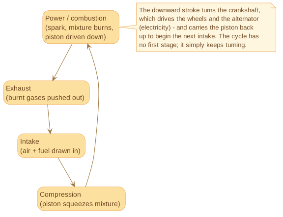
Such a map lets you see at a glance how the stages of an engine feed one another to produce power and electricity. Describing the same cycle in words would take far longer and, most likely, leave you with a weaker picture of how the whole thing turns.

Decision Trees#

When a decision involves uncertainty and real stakes, it helps to lay out the choices, the things that could happen after each choice, and what each outcome is worth – all on one diagram – before you commit money, time and people. That’s a decision tree. Where you can put numbers on the payoffs and the odds, the tree also lets you compute which option is best on average; where you can’t, it still forces the options and their consequences into the open. Below is a worked example. A bottled-water company has to decide whether to do market research before launching a new product aimed at high-performing students. The dollar amounts are in thousands of dollars (‘000s’).

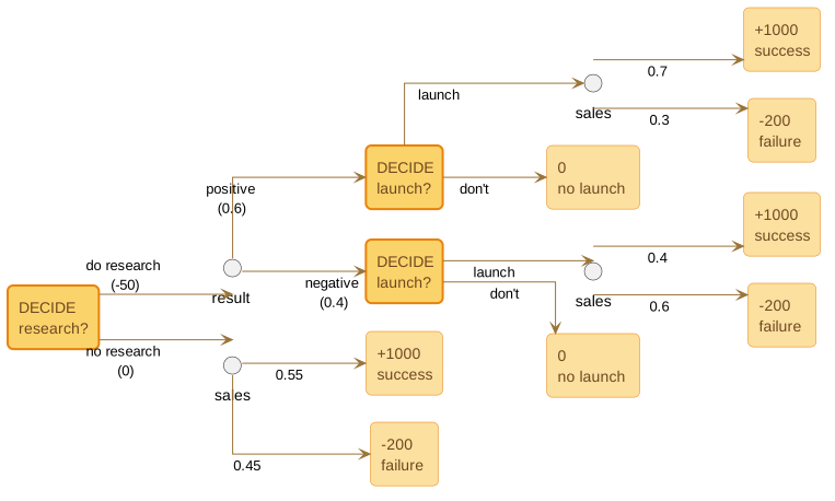
Each option branches into the things that could follow it, and each of those branches into the costs and possible outcomes. This is usually the first of a series of trees – as you learn more, you revise it, add variables you’d missed, and re-run the numbers. It’s a tool for thinking, not a one-shot oracle.

Run the numbers on this particular tree and they point one way: the company is better off not doing market research. Let’s see how that falls out.

Constructing a decision tree#

A decision tree has two kinds of node. A decision node (drawn as a square) is a choice you control. An event node, also called a chance node (drawn as a circle), is an outcome you don’t control. Let’s look at each. Here’s a decision node:

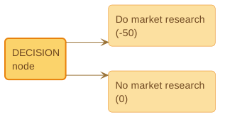
Here the company has two choices – do market research or don’t. Research costs $50,000, so you write that as a negative amount on its branch. Not doing research costs nothing. Now an event node:

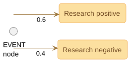
If the company does the research, history says it comes back positive about 60% of the time and negative 40% of the time. You write these probabilities – 0.6 and 0.4 – on the branches leaving the chance node. (The probabilities on any one chance node must add up to 1.)

You build the tree from these parts first, then calculate it, working “forwards, then backwards.” Let’s follow one whole branch:

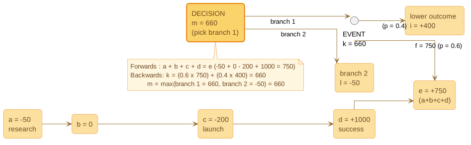
Working forwards means adding the figures along each branch to get its total payoff. Above, a+b+c+d gives e: (-50) + 0 + (-200) + 1000 = $750. So if the company does research and the product succeeds, that path is worth $750,000.

Working backwards uses the probabilities to fold the uncertain nodes into a single number – the expected monetary value (EMV). You write the result below each node:

• At an event (chance) node – point k above – you take a probability-weighted average of its branches: k = (0.6 x 750) + (0.4 x 400) = 660. The EMV is what you’d get on average if you faced this same gamble many times; it is not what you’ll get on any single launch.

• At a decision node – point m above – you don’t average. You’re in control here, so you simply pick the better branch and carry its value up. Branch 1 (660) beats branch 2 (-50), so you mark branch 1 and write 660 at m.

You keep folding backwards, node by node, until you reach the left-hand side. The branches you picked along the way trace out the highest-EMV path.

Go back to the tree at the start of this section. Which path do the numbers favour? Do no market research, and launch.

Two honest caveats. First, EMV is an average, so it’s the right rule when you’ll face many similar decisions, but it can mislead on a single bet-the-company call where one bad outcome would sink you – there, the spread of outcomes matters as much as the average. Second, the tree above only counts money. Real decisions carry effects a payoff column misses: a product failure could dent “corporate image,” and that could quietly cost you sales across the whole range. A decision tree is only as good as the payoffs, probabilities and factors you feed it – garbage in, garbage out.

With those caveats, decision trees earn their keep well beyond business. You can use the same structure to think through changing jobs, where to live, or what to study – anywhere you face a choice with uncertain consequences and want to see them laid out rather than churning in your head.

From decision diagram to runnable logic#

A decision tree weighs uncertain options with probabilities. A closely related diagram, the decision flowchart, captures a rule: given some facts, follow the yes/no branches to a decision. You draw one to learn a policy – how a triage nurse sorts patients, how a loan is approved, how our bottled-water company decides whether to launch:

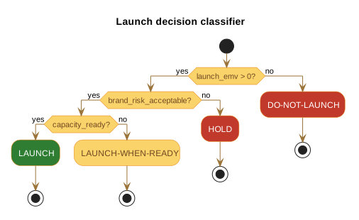
Here’s something worth knowing once you’ve drawn one: a decision flowchart like this isn’t only a picture. Draw it in PlantUML – a plain-text way of writing diagrams – and a small open-source tool called clearlogic (by ClearKan, a sibling project living at ../clearlogic) will compile it into runnable code: a deterministic classifier that takes the same inputs and returns the same decision, every time, with no AI in the loop. The diagram above is exactly that subset – it compiles, and it answers correctly for each path through the chart. clearlogic does the same for state diagrams, the kind that model a thing moving through stages (an order: placed -> paid -> shipped -> delivered).

The idea behind it is the same cybernetic thread running through this whole module: the visible flow is the policy. When the picture you can read and the rule the machine runs are the same artefact, there’s nothing hidden between what you understand and what executes – you can inspect it, diff it, and audit it. So the practical upshot for a learner is simply this: learn the diagram here; when you later need it to actually run, it already can. That’s it – no need to oversell it. Most maps in this course are for thinking. A decision flowchart can be for thinking and for doing.

Logic Trees#

A logic tree is a diagram that starts with a key statement and then branches out with further logic or key points that support the statement. There are two types of reasoning—deductive and inductive—that you can use to establish logical relationships between ideas. Let’s look at each of these types in turn.

Deductive reasoning#

Deductive reasoning moves from things you know or assume to be true – the ‘premises’ – to a conclusion that must follow from them. It leads to a “therefore.” Here’s a simple example:

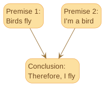
The first two statements are premises (Birds fly, I’m a bird); the third is the conclusion (Therefore, I fly). By the rules of deduction, if the premises are true, the conclusion must be true. (Whether the premises actually are true is a separate question – “birds fly” lets in penguins. Deduction guarantees the link, not the inputs.) Any deductive argument needs to do three things:

• Make a statement about something that exists in the world; i.e., Birds fly.

• Make another statement about a related situation that exists in the world at the same time: i.e., I’m a bird. The second statement relates to the first if it comments on either its subject (birds) or its predicate (fly).

• State the implication of these two situations existing in the world at the same time; i.e., Therefore, I fly.

Deductive statements can sometimes become too long and boring if you include every step included in the process. In cases like that, you can skip a step and “chain together” two or more deductive arguments. Here’s an example: Assume that the issue under consideration is aluminum production in Australia. The deductive argument might look like this in text form:

• Australia produces enough aluminum to meet its own needs.

• But exports to Asia have increased, reducing supply to below domestic demand.

• Therefore, Australia has a shortage.

• A shortage of aluminum causes a shortage of manufactured goods.

• We have a shortage of aluminum.

• Therefore, there is a shortage of manufactured goods.

That’s a lot of steps. If you skip and consolidate some of them, you get a “chained” deductive argument that looks like this as a map:

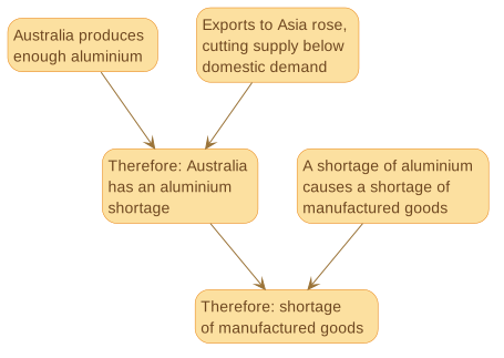
The key in deciding whether to use a chained deductive argument is this: The reader must be able to understand the missing steps and agree with them.

Inductive reasoning#

The second type of reasoning is inductive. Here you move from a set of examples to a general theory you think explains them – and the examples still to come. Induction tends to be more creative than deduction’s “straight-ahead” logic, because your mind has to notice that several separate things are alike in some way, group them, and say why the similarity matters. Here’s an inductive argument as a map:

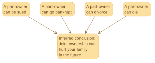
Reading the map, you infer from the four lower nodes a single conclusion: joint ownership can hurt your family later on.

Here’s the crucial difference. A deductive conclusion must be true if its premises are. An inductive conclusion may or may not be – it’s a reasonable bet, not a guarantee. Visit rainy Seattle for a few days and it might rain every day you’re there; you could infer it rains every day in Seattle. You’d be wrong. It rains a lot there, but not every day. Induction reaches beyond the examples it’s built on, and that reach is exactly where it can fail – so treat an induced conclusion as a hypothesis to keep testing, not a settled fact.

Using logic trees#

Logic trees turn up across maths, logic, computer science and law – and they’re a practical way to build the backbone of a report or presentation. Look at this diagram:

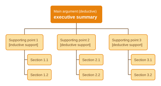
This diagram shows the structure of a logical argument. The main argument at the top is deductive; however, lower level arguments support each higher point. An inductive argument supports the first point, whereas deductive arguments support the next two points.

Once you have your argument laid out like this, you can then structure your report or presentation along the same lines. The top point is your executive summary; the second level points become chapters; and the third and fourth levels become sections within those chapters.

Software-based concept maps#

Everything so far you can draw by hand. This last group of maps is different: they exist because of software, which can lay out, filter and animate far more information than you could ever arrange on paper. They’re worth knowing as a category — when a map grows too big or too dynamic to draw, reach for a tool. (For the tools themselves, see Software for concept mapping .)

A few kinds you’ll come across:

• Automated and force-directed layouts. The software positions concepts for you, modelling each link as a force that pulls related ideas together and pushes unrelated ones apart. Drag one node and the whole map reflows. This is how the “graph view” in note tools like Obsidian, and dedicated graph tools, reveal the shape of a large knowledge base at a glance.

• Hyperbolic or “fisheye” trees. A focus-and-context view for big hierarchies: whatever you point at grows and spreads out while distant branches shrink to the edges, so you keep your bearings without endless zooming. Handy for navigating large sites, file systems, or taxonomies.

• Treemaps. Instead of nodes and lines, these pack nested rectangles whose size and colour encode quantity and change — letting you compare thousands of items (budgets, disk usage, categories of anything) in a single view and drill down with a click.

• 3D and interactive models. For structures a flat diagram can’t capture — a molecule’s shape, say — a rotatable 3D model is itself a kind of concept map, with the parts as concepts and the bonds as links. Open-source viewers like Jmol/JSmol and Mol* do this for chemistry; the same idea shows up in any field with spatial structure.

The frontier has moved on since this course was first written: force-directed graphs, treemaps and 3D views are now built into everyday note apps and analytics tools, and AI can draft a map from your notes — or restructure one as you learn. The principle hasn’t changed, though. Software earns its place only when a map is too large, too connected, or too dynamic to hold on a page. For everything else, a pen still wins.

Other types of maps#

Here is a brief summary of other concept maps you might want to investigate further.

• Gantt charts and PERT charts. Project managers often use these charts to model the sequence of tasks over time. Links between tasks show dependencies, and positions of tasks show when the tasks should occur. Various other visual elements show task completeness, delays in schedule, overruns and other information.

• Data Flow Diagrams and Entity Relationship Diagrams. These diagrams model the flow of data in a computer system or database. Computer professionals use these to design and communicate information about computer software.

Summary#

Systems concept maps show the cycle, or cycles, in a system, letting you hold a whole dynamic system on one page rather than just its parts. Their real subject is feedback: balancing loops that seek a goal and hold it (the bucket, a thermostat), reinforcing loops that amplify a change (compound interest), and the delays that make systems oscillate (the shower). Drawn as causal-loop diagrams, they’re the working tool of systems thinking and cybernetics – and the same lens applies to learning, which is itself a feedback loop. Logic trees start with a key statement and branch into the points that support it, built from two kinds of reasoning: deductive (premises that force a “therefore” conclusion – guaranteed if the premises hold) and inductive (examples that suggest a general theory – a reasonable bet, not a guarantee). Decision trees lay out a choice and its uncertain outcomes so you can weigh them before committing time, money and people; where you know the payoffs and probabilities, folding the tree backwards gives each option an expected monetary value – an average, not a promise about any single outcome. They’re built from decision nodes (a choice you control) and event nodes (an outcome you don’t). A decision flowchart – the rule-based cousin – can go one step further: written in PlantUML, it compiles to runnable, deterministic code, so the diagram you read is the policy that executes. Software-based concept maps use the power of computers to lay out, filter and animate more than you could ever arrange by hand – worth reaching for when a map grows too big or too dynamic for paper, and otherwise not.

Exercises#

Exercise 1 - Deductive Logic concept map#

Construct a visual logic map from the following information about a company:

• Any corporation meeting three specific criteria is worth buying.

• Company X meets all three criteria.

Remember, a deductive logic concept map must follow three criteria:

• Make a statement about something that exists in the world; i.e., Birds fly.

• Make another statement about a related situation that exists in the world at the same time: i.e., I’m a bird. The second statement relates to the first if it comments on either its subject (birds) or its predicate (fly).

• State the implication of these two situations existing in the world at the same time; i.e., Therefore, I fly.

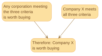
Suggested solution. The two pieces of information map straight onto the three-part deductive pattern. The first statement is the general rule — any corporation meeting the three criteria is worth buying. The second is the matching case — Company X meets all three criteria. Both are premises, so they sit side by side and point to the single conclusion that must follow: therefore, Company X is worth buying. It’s the same shape as Birds fly / I’m a bird / Therefore I fly — two premises feeding one “therefore”. As with every map in this course, this is a guide, not the only correct answer: you might phrase the nodes differently or spell out the three criteria, and that’s fine.